Outline
Outline
- Why Word Vectors?
- GloVe Model
- Evaluating GloVe
- About the Data
- Evaluation of real Word Vectors
- Outlook
- Conclusion
Why Word Vectors?
Mathematical Representation of Words
- Map of each word \(i\) to a corresponding word vector \(w_i \in \mathbb{R}^d\) (word embedding).
- The word vector \(w_i\) can be used to do further analyses e. g. clustering or as input for more sophisticated text mining models.
- Of course we want to have useful word vectors \(w_i\):
- A dimension one can work on (dimensional reduction).
- Representation of the human understanding of words.
\(\rightarrow\) GloVe is a model which constructs word vectors out of a given corpus.
Goal of GloVe
Model word semantic and analogies between words. Therefore, it is very important to constitute a linear structure of the word vector space. The following graphic was created using 3 dimensional word vectors trained with GloVe:
GloVe Model
About GloVe
GloVe was introduced by Jeffrey Pennington, Richard Socher and Christopher D.Manning [Pennington et al. 2014]:
" … GloVe is an unsupervised learning algorithm for obtaining vector representations for words. Training is performed on aggregated global word-word co-occurrence statistics from a corpus, and the resulting representations showcase interesting linear substructures of the word vector space."
Theory: word-word co-occurence Matrix
Base of the model is the word-word co-occurrence matrix \(X \in \mathbb{R}^{|V| \times |V|}\), where \(|V|\) is the number of different words which occurs within a given corpus. In \(X\) every entry \(X_{ij}\) describes how often word \(j\) occurs in context of word \(i\) with a given window size. Therefore we have the following properties:
\(X_i = \sum_k X_{ik}\): Number of words which occur in the context of \(i\).
\(P_{ij} = P(j | i) = X_{ij} / X_i\): "Probability" of word \(j\) occurs in context of \(i\).
- The ratio \(P_{ik} / P_{jk}\) describes if word \(k\) is more related to …
- … word \(i\) if \(P_{ik} / P_{jk} > 1\)
- … word \(j\) if \(P_{ik} / P_{jk} < 1\)
- … or similar related if \(P_{ik} / P_{jk} \approx 1\)
Example: word-word co-occurenece Matrix
Corpus:
Window size:
word-word co-occurenece matrix:
\[ \begin{array}{c|ccccc} & \text{A} & \text{B} & \text{C} & \text{D} & \text{E} \\ \hline \text{A} & 0 & 1 & 3 & 2 & 4 \\ \text{B} & 1 & 0 & 1 & 1 & 1 \\ \text{C} & 3 & 1 & 0 & 2 & 2 \\ \text{D} & 2 & 1 & 2 & 0 & 4 \\ \text{E} & 4 & 1 & 2 & 4 & 0 \end{array} \ \ \Rightarrow\ \ P_\text{AD} = X_\text{AD} / X_\text{A} = \frac{2}{10} \]
Where to Start?
Remember: We want to create word vectors \(w_i \in \mathbb{R}^d\) and want to use the ratio \(P_{ik} / P_{jk}\) since the ratio is more appropriate to take words into context.
The Idea:
\[ F(w_i, w_j, \tilde{w}_k) = \frac{P_{ik}}{P_{jk}} \]
with word vectors \(w_i, w_j\) and context vector \(\tilde{w}_k\). \(F\) is unknown at this stage and basically can be any function.
We now parameterize every word vectors, therefore we have \(d \cdot |V|\) parameter to estimate to get word vectors.
How does \(F\) looks like?
Reduce number of possible outputs of \(F\) by taking \(w_i - w_j\) instead of two vectors \(w_i\) and \(w_j\): \[ F(w_i - w_j, \tilde{w}_k) = \frac{P_{ik}}{P_{jk}} \]
We want to keep the linear structure between the word vectors and context vector: \[ F\left((w_i - w_j)^T\tilde{w}_k\right) = \frac{P_{ik}}{P_{jk}} \]
Keep exchange symmetry. We want be able to exchange word vectors \(w\) with context vectors \(\tilde{w}\) without getting different results:
\(\rightarrow\) Not given at this stage.
How does \(F\) looks like?
To find \(F\) and obtain the exchange symmetry we need to apply two "tricks":
- We restrict \(F\) to be a homomorphism between \((\mathbb{R}, f) = (\mathbb{R}, +)\) and \((\mathbb{R}_+, g) = (\mathbb{R}_+, \cdot )\). That means we expect \(F\) to fulfill: \[
F(a + b) = \underbrace{F(f(a, b)) = g(F(a), F(b))}_{\text{Definition of homomorphism}} = F(a)F(b)
\] With \(a = w_i^T\tilde{w}_k\) and \(b = -w_j^T\tilde{w}_k\).
We notice, that the upper equation implies a functional equation which has just one solution: \[ F = \exp_a \]
How does \(F\) looks like?
To find \(F\) and obtain the exchange symmetry we need to apply two "tricks":
- We choose \(a = \exp(1)\), therefore \(F = \exp\). \[ F\left((w_i - w_j)^T\tilde{w}_k\right) = \exp\left((w_i - w_j)^T\tilde{w}_k\right) = \frac{\exp(w_i^T\tilde{w}_k)}{\exp(w_j^T\tilde{w}_k)} = \frac{P_{ik}}{P_{jk}} \\ \Rightarrow\ \exp(w_i^T\tilde{w}_k) = P_{ik} = \frac{X_{ik}}{X_i} \\ \Leftrightarrow\ w_i^T\tilde{w}_k = \log(X_{ik}) - \log(X_i) \\ \Leftrightarrow\ w_i^T\tilde{w}_k + \log(X_i) = \log(X_{ik}) \] But: How to handle \(X_{ik} = 0\)? We handle this later.
How does \(F\) looks like?
To find \(F\) and obtain the exchange symmetry we need to apply two "tricks":
- Since \(\log(X_i)\) is independent of \(k\) we can put this in a bias term. This bias term can be decomposed into a term \(b_i\) from \(w_i\) and \(\tilde{b}_k\) from \(\tilde{w}_k\): \[ \Rightarrow\ w_i^T\tilde{w}_k + b_i + \tilde{b}_k = \log(X_{ik}) \] This is now an model equation which we can use for training the word vectors. We also note, that we have transformed the unsupervised task into a supervised task which we know how to handle.
Model Equation
A problem appears for \(X_{ik} = 0\). This is definitely the case since \(X\) is a sparse matrix. We don't want to drop the sparsity due to convenient memory handling. Therefore, we use an additive shift in the logarithm: \[ \log(X_{ik})\ \rightarrow\ \log(X_{ik} + 1) \] This maintains the sparsity: \[ X_{ik} = 0\ \Rightarrow\ \log(X_{ik} + 1) = \log(1) = 0 \] The final model equation which we use for training is \[ w_i^T\tilde{w}_k + b_i + \tilde{b}_k = \log(X_{ik} + 1) \]
Empirical Risk
To estimate the word vectors GloVe uses a weighted least squares approach: \[ J = \sum\limits_{i=1}^{|V|}\sum\limits_{j=1}^{|V|}f(X_{ij})\left(w_i^T\tilde{w}_j + b_i + \tilde{b}_j - \log(X_{ij} + 1)\right)^2 \] [Pennington et al. 2014] proposed as weight function: \[ f(x) = \left\{ \begin{array}{ccc} (x / x_\mathrm{max})^\alpha, & x < x_\mathrm{max} \\ 1, & x \geq x_\mathrm{max} \end{array} \right. \]
Using this function also introduces two new hyperparameters \(\alpha\) and \(x_\mathrm{max}\). The ordinary way to find good values for \(\alpha\) and \(x_\mathrm{max}\) would be to use a tuning method. The problem now is that for all tuning methods we need to evaluate the model. Since we want to handle an unsupervised task evaluating isn't straightforward.
Algorithm used for Fitting
Basically, GloVe uses a gradient descend technique to minimize the objective \(J\). Nevertheless, using ordinary gradient descend would be way too expensive in practice. Therefore some adoptions:
Individual learning rate in each iteration.
Adaption of the learning rate to the parameters, performing larger updates for infrequent and smaller updates for frequent parameter.
Well-suited for sparse data, improve robustness of (stochastic) gradient descent.
For GloVe, infrequent words require much larger updates than frequent ones.
\(\rightarrow\) AdaGrad meets these requirements.
What to do with Word Vectors?
Evaluating GloVe
Evaluation: Metrics
We need something to measure the distance between vectors:
Euclidean Distance \[ d_\mathrm{euclid}(x,y) = \sqrt{\sum\limits_{i=1}^n(x_i - y_i)^2} \]
Cosine Distance \[ d_\mathrm{cosine}(x,y) = 1 - \mathrm{cos}(\angle (x, y)) = 1 - \underbrace{\frac{\langle x,y\rangle}{\|x\|_2\|y\|_2}}_{\mathrm{Cosine\ Similarity}} \]
In general we could use every metric to evaluate the model. But the cosine similarity is more robust in terms of curse of dimensionality.
Evaluation: p-Norm in high Dimensions
[Aggarwal et al. 2001] have shown, that in high dimensions the ratio of the maximal norm divided by the minimal norm of \(n\) points \(x_1, \dots, x_n\) which are randomly drawn converges in probability to 1 for increasing dimension \(d\): \[ \underset{{d\rightarrow\infty}}{\mathrm{p~lim}}\ \frac{\mathrm{max}_k \|x_k\|_2}{\mathrm{min}_k \|x_k\|_2} = 1 \]
\(\Rightarrow\) Points are concentrated on the surface of a hyper sphere using the
euclidean norm.
The same holds for every \(p\)-Norm.
Evaluation: p-Norm in high Dimensions
Evaluation: Semantic and Analogies
One thing we now can do is to ask for semantic analogies between words. Something like: \[ \mathrm{paris\ behaves\ to\ france\ like\ berlin\ to\ ?} \\ \mathrm{animal\ behaves\ to\ animals\ like\ people\ to\ ?} \\ \mathrm{i\ behaves\ to\ j\ like\ k\ to\ l} \] Therefore, we have \(3\) given word vectors \(w_i\), \(w_j\) and \(w_k\). To get the desired fourth word \(l\) we use the linearity of the word vector space: \[ w_l \approx w_j - w_i + w_k \] Furthermore, we obtain \(\widehat{l}\) from our model and a given metric \(d(w_i, w_j)\) (mostly \(d = d_\mathrm{cosine}\)) by computing: \[ \widehat{l} = \underset{l \in V}{\mathrm{arg~min}}\ d(w_j - w_i + w_k, w_l) \]
Evaluation: Questions Words File
To evaluate trained word vectors, [Mikolov et al. 2013] provide a word similarity task. This task is given within a question words file which contains about 19544 semantic analogies:
Evaluation: Question Words File
| Category | Number of Test Lines | Example |
|---|---|---|
| capital-common-countries | 506 | Athens Greece Baghdad Iraq |
| capital-world | 4524 | Abuja Nigeria Accra Ghana |
| currency | 866 | Algeria dinar Angola kwanza |
| city-in-state | 2467 | Chicago Illinois Houston Texas |
| family | 506 | boy girl brother sister |
| gram1-adjective-to-adverb | 992 | amazing amazingly apparent apparently |
| gram2-opposite | 812 | acceptable unacceptable aware unaware |
| gram3-comparative | 1332 | bad worse big bigger |
| gram4-superlative | 1122 | bad worst big biggest |
| gram5-present-participle | 1056 | code coding dance dancing |
| gram6-nationality-adjective | 1599 | Albania Albanian Argentina Argentinean |
| gram7-past-tense | 1560 | dancing danced decreasing decreased |
| gram8-plural | 1332 | banana bananas bird birds |
| gram9-plural-verbs | 870 | decrease decreases describe describes |
Evaluation: Hyperparamter Tuning
Now tuning is "possible" for a given task specified in the questions words file.
- [Pennington et al. 2014] have tuned the model and came to good values (just empirical without a proof):
- \(\alpha = 0.75\)
- \(x_\mathrm{max} = 100\) (does just have a weakly influence on performance)
Note that we are dependent on this file and can just test on this file. If we want to test other properties of the model we need other files.
About the Data
Data: The Language
- Be careful with the language:
| German term list | English term list |
|---|---|
| Wassermolekuel | hydrogen |
| Wasserstoff | hydrogen-bonding |
| Wasserstoffatom | |
| Wasserstoffbindung | |
| Wasserstoffbrueckenbildung | |
| Wasserstoffbrueckenbindung | |
| Wasserstoffhalogenid | |
| Wasserstoffverbindung |
Copied from Grammar & Corpora 2009 [Konopka 2011]. Excerpt of the resulting English and German term lists focusing on the term hydrogen (German: Wasserstoff).
For instance, German has much more rare words and a bigger variety (harder for modelling) than English.
Data: The Corpus
We need a lot of words to train the model.
Often crawled from the web. This is mostly followed by a lot of preprocessing (regular expressions, filtering stop words etc.).
How big should the corpus and the vocabular be to get good word vectors?
Does different corpora imply a different quality of the word vectors?
Data: Common Sources
Wikipedia Dump + Gigaword 5: Wikipedia gives access to all articles collected within one XML file (unzipped about 63 GB). [Pennington et al. 2014] combines this with Gigaword 5, an archive of newswire text data.
\(\rightarrow\) 6 billion tokens and 400 thousand word vocabularyCommon Crawl: Published by Amazon Web Services through its Public Data Sets program in 2012. The data was crawled from the whole web and contains 2.9 billion web pages and over 240 TB of data.
\(\rightarrow\) 42 billion tokens and 1.9 million word vocabulary or
\(\rightarrow\) 820 billion tokens and 2.2 million word vocabularyTwitter: [Pennington et al. 2014] crawled 2 billion tweets.
\(\rightarrow\) 27 billion tokens and 1.2 million word vocabulary
Evaluation of real Word Vectors
Training Word Vectors
Train word vectors using …
the
Rpackagetext2vec[Selivanov and Wang 2017].the full Wikipedia dump with first 453.77 million words (16 %, due to memory consumption).
- the same settings as [Pennington et al. 2014]:
- \(\alpha = 0.75\)
- \(x_\mathrm{max} = 100\)
- Learning rate of \(0.05\)
- \(\mathrm{Number\ of\ iterations} = \left\{\begin{array}{cc} 50 & \text{if} \ d < 300 \\ 100 & \text{otherwise} \end{array}\right.\).
a more advanced text pre processing (stopwords etc.).
Own Word Vectors
Own word vectors fitted on the Wikipedia dump:
| Category | Number of Test Lines | 25 d | 50 d | 100 d | 200 d | 300 d |
|---|---|---|---|---|---|---|
| capital-common-countries | 506 | 0.3715 | 0.6739 | 0.8636 | 0.8715 | 0.8854 |
| capital-world | 4524 | 0.1461 | 0.3333 | 0.4657 | 0.4348 | 0.4726 |
| currency | 866 | 0.0035 | 0.0127 | 0.0173 | 0.0231 | 0.0150 |
| city-in-state | 2467 | 0.1110 | 0.2345 | 0.4191 | 0.4664 | 0.5306 |
| family | 506 | 0.3794 | 0.5474 | 0.6186 | 0.6047 | 0.6344 |
| gram1-adjective-to-adverb | 992 | 0.0554 | 0.1562 | 0.2006 | 0.1925 | 0.1986 |
| gram2-opposite | 812 | 0.0222 | 0.0480 | 0.1195 | 0.1527 | 0.1884 |
| gram3-comparative | 1332 | 0.3033 | 0.4775 | 0.6329 | 0.7065 | 0.7680 |
| gram4-superlative | 1122 | 0.0784 | 0.1613 | 0.2843 | 0.3084 | 0.3422 |
| gram5-present-participle | 1056 | 0.2377 | 0.3191 | 0.4186 | 0.4934 | 0.5625 |
| gram6-nationality-adjective | 1599 | 0.5358 | 0.7199 | 0.8054 | 0.8554 | 0.8698 |
| gram7-past-tense | 1560 | 0.2032 | 0.3436 | 0.4609 | 0.5385 | 0.5532 |
| gram8-plural | 1332 | 0.3326 | 0.6051 | 0.7568 | 0.8303 | 0.8116 |
| gram9-plural-verbs | 870 | 0.1793 | 0.2713 | 0.4149 | 0.4977 | 0.5402 |
| Accuracy | 0.1992 | 0.3469 | 0.4688 | 0.4989 | 0.5300 |
Pre-Trained Word Vectors
| Wikipedia + Gigaword 5 | Common Crawl | |||||||||
|---|---|---|---|---|---|---|---|---|---|---|
| Category | Number of Test Lines | 50 d | 100 d | 200 d | 300 d | 300 d | 25 d | 50 d | 100 d | 200 d |
| capital-common-countries | 506 | 0.7984 | 0.9407 | 0.9526 | 0.9545 | 0.9466 | 0.1502 | 0.2688 | 0.5178 | 0.6477 |
| capital-world | 4524 | 0.6877 | 0.8840 | 0.9421 | 0.9598 | 0.9229 | 0.0969 | 0.2452 | 0.5050 | 0.6796 |
| currency | 866 | 0.0866 | 0.1455 | 0.1663 | 0.1617 | 0.1663 | 0.0000 | 0.0080 | 0.0120 | 0.0199 |
| city-in-state | 2467 | 0.1585 | 0.3020 | 0.5071 | 0.6044 | 0.7815 | 0.0243 | 0.0669 | 0.1767 | 0.3522 |
| family | 506 | 0.7016 | 0.8004 | 0.8360 | 0.8775 | 0.9130 | 0.3063 | 0.4565 | 0.5929 | 0.6660 |
| gram1-adjective-to-adverb | 992 | 0.1361 | 0.2359 | 0.2500 | 0.2248 | 0.2913 | 0.0131 | 0.0343 | 0.0746 | 0.1159 |
| gram2-opposite | 812 | 0.0924 | 0.2020 | 0.2365 | 0.2685 | 0.3374 | 0.0582 | 0.0913 | 0.1865 | 0.2447 |
| gram3-comparative | 1332 | 0.5375 | 0.7905 | 0.8566 | 0.8724 | 0.8566 | 0.1682 | 0.4429 | 0.6306 | 0.7342 |
| gram4-superlative | 1122 | 0.2834 | 0.5490 | 0.6756 | 0.7077 | 0.8601 | 0.1542 | 0.3734 | 0.5570 | 0.5998 |
| gram5-present-participle | 1056 | 0.4167 | 0.6884 | 0.6752 | 0.6951 | 0.8002 | 0.2074 | 0.4706 | 0.6136 | 0.6553 |
| gram6-nationality-adjective | 1599 | 0.8630 | 0.8856 | 0.9243 | 0.9256 | 0.8799 | 0.1427 | 0.3024 | 0.4799 | 0.6160 |
| gram7-past-tense | 1560 | 0.3596 | 0.5340 | 0.5859 | 0.5962 | 0.4910 | 0.1737 | 0.3532 | 0.4923 | 0.5051 |
| gram8-plural | 1332 | 0.5901 | 0.7162 | 0.7718 | 0.7785 | 0.8401 | 0.2020 | 0.4932 | 0.6441 | 0.7575 |
| gram9-plural-verbs | 870 | 0.3805 | 0.5839 | 0.5954 | 0.5851 | 0.6425 | 0.1885 | 0.4034 | 0.5460 | 0.5241 |
| Accuracy | 0.4645 | 0.6271 | 0.6934 | 0.7157 | 0.7472 | 0.1212 | 0.2744 | 0.4358 | 0.5385 | |
Accuracy of Word Vectors
Outlook
Outlook: Text Classification
- An example is text classification for which word embeddings can be used to map text to an image:
1st Step: Imagine the following word vectors obtained by GloVe: \[ \begin{array}{c|ccc} A & 0.1 & 0.2 & 0.1 \\ B & 0.2 & 0.5 & 0.3 \\ C & 0.9 & 0.7 & 0.3 \\ D & 0.4 & 0.8 & 0.1 \end{array} \ \ \Rightarrow \ \ w_i \in \mathbb{R}^3, \ d = 3 \]
Note that word vectors created by GloVe are organized as rows within the matrix where the rownames displays the vocabulary of available words.
Outlook: Text Classification
- An example is text classification for which word embeddings can be used to map text to an image:
2nd Step: Now we have a given text: \[ \mathrm{A\ B\ A\ D\ B\ C} \]
Outlook: Text Classification
- An example is text classification for which word embeddings can be used to map text to an image:
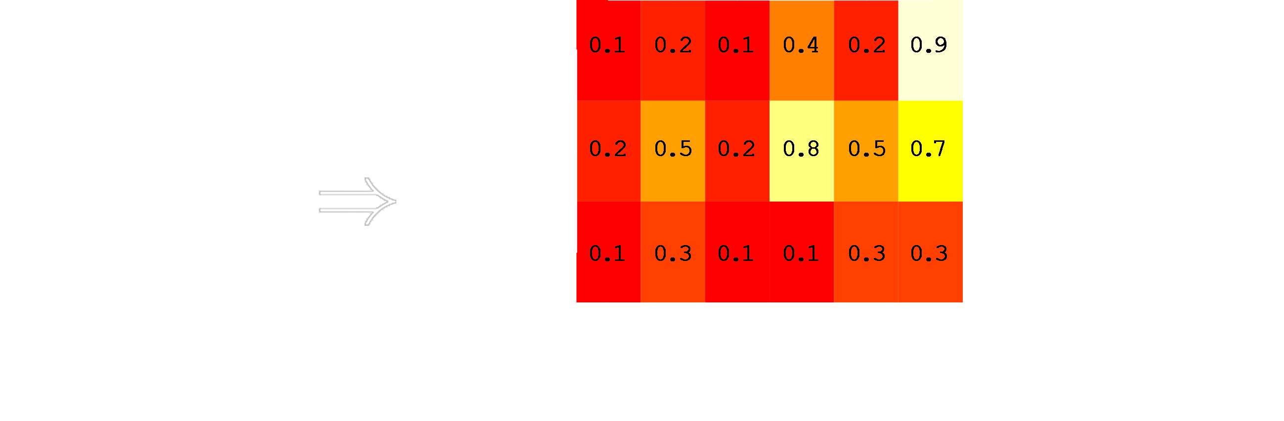
3rd Step: Next, each word in the text is mapped to the corresponding word vector to obtain a matrix for the given text: \[ \begin{array}{cccccc} \mathrm{A} & \mathrm{B} & \mathrm{A} & \mathrm{D} & \mathrm{B} & \mathrm{C} \\ \downarrow & \downarrow & \downarrow & \downarrow & \downarrow & \downarrow \\ 0.1 & 0.2 & 0.1 & 0.4 & 0.2 & 0.9 \\ 0.2 & 0.5 & 0.2 & 0.8 & 0.5 & 0.7 \\ 0.1 & 0.3 & 0.1 & 0.1 & 0.3 & 0.3 \end{array} \]
Outlook: Text Classification
- An example is text classification for which word embeddings can be used to map text to an image:
4th Step: This matrix can be used to create an image out of the given text by translating the matrix to an image:
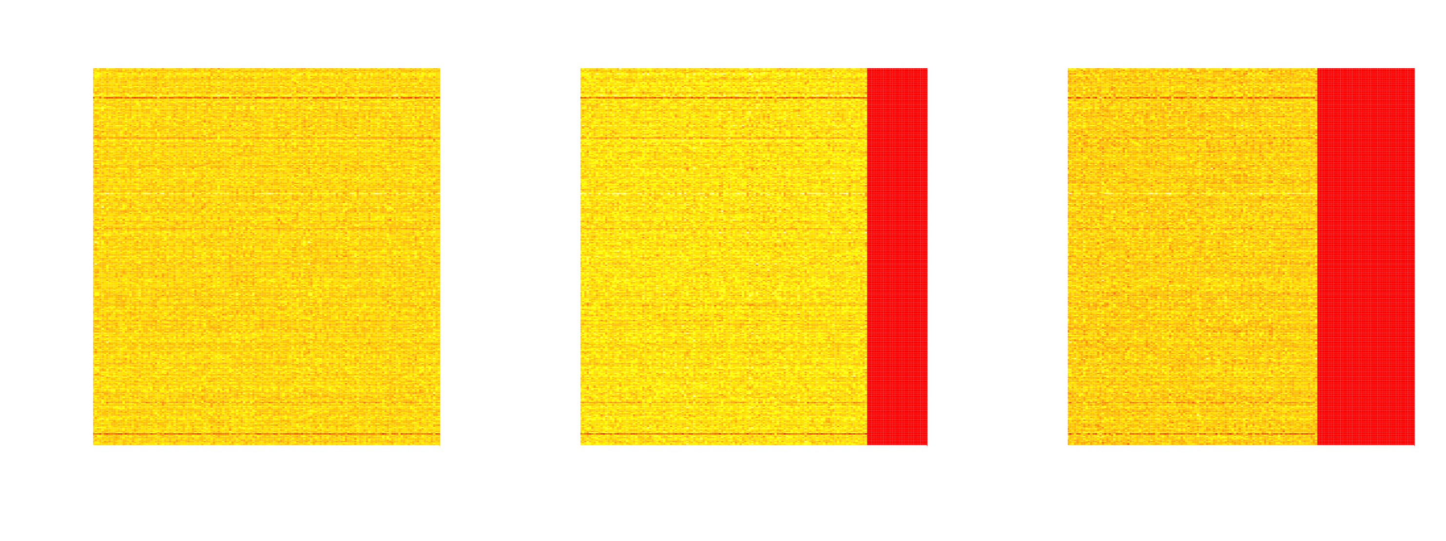
Outlook: Text Classification
The following images were generated from the introduction of Principia Mathematica by Sir Isaac Newton and Elements of Statistical Learning, as well as from Sonnet 18 by William Shakespear:
Conclusion
Conclusion
With GloVe it is possible to create meaningful word embeddings.
[Pennington et al. 2014] compared several models on the word analogy task, whereas GloVe outperforms the others.
But accuracy of word analogy task depends not only on the dimension, but also on the corpus.
Use servers or pcs with huge computing power to train GloVe due to the need of huge corpora an computing time!
References
References
Aggarwal, C. C., Hinneburg, A., and Keim, D. A. [2001], “On the surprising behavior of distance metrics in high dimensional space,” in International conference on database theory, Springer, pp. 420–434.
Konopka, M. [2011], Grammar & corpora 2009, BoD–Books on Demand.
Mikolov, T., Chen, K., Corrado, G., and Dean, J. [2013], “Efficient estimation of word representations in vector space.”
Pennington, J., Socher, R., and D. Manning, C. [2014], “GloVe: Global vectors for word representation,” in Empirical methods in natural language processing (emnlp), pp. 1532–1543.
Selivanov, D., and Wang, Q. [2017], Text2vec: Modern text mining framework for r.